Table Of Content
Now let us introduce a machine drift (Figure Figure11C,G) that causesthe mass spectrometer todetect slightly less of the protein over time. For the ordered allocation,the observed protein abundances show almost no difference betweenthe two group means (Figure Figure11D). Conversely, the difference in group means for the randomizedallocation is nearly the same as the “true” difference(Figure Figure11H), and onlyhas added variance caused by the machine drift (Figure Figure22).
Continuous Variables and
Our global experiments past, present and future - Royal Society of Chemistry
Our global experiments past, present and future.
Posted: Wed, 27 Mar 2019 02:32:25 GMT [source]
We now illustrate the GLM analysis based on the missing data situation - one observation missing (Batch 4, pressure 2 data point removed). The least squares means as you can see (below) are slightly different, for pressure 8700. What you also want to notice is the standard error of these means, i.e., the S.E., for the second treatment is slightly larger.
Summary
In a completely randomized $2\times2$ factorial layout (no blocks), you would completely randomly decide the order in which the breads are baked. For each loaf, you would preheat the oven, open a package of bread dough, and bake it. This would involve running the oven 160 times, once for each loaf of bread. Graphical exploration of the data is a little more problematic in this example. As each treatment does not occur in each block, box plots such as Figure 3.2 are not as informative. Do compounds three and four have higher average wear because they were the only compounds to both occur in blocks 3 and 4?
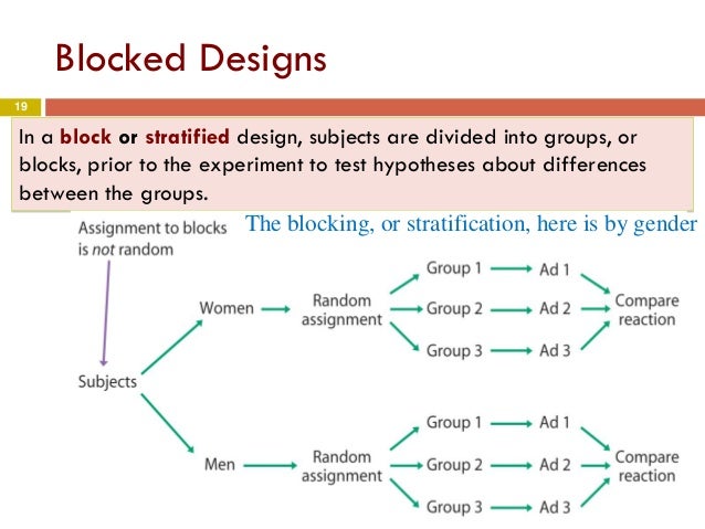
2.4 Evaluating and Choosing a Blocking Factor

We note that the sum of squares and the mean square estimates are slightly larger than for the aov() analysis, because the between-block information is taken into account. This provides more power and results in a slightly larger value of the \(F\)-statistic. Note that the categorized version is solely created forblock allocation, and the final analysis still uses the original variable. The strategiesoutlined for the theoretical settings above caneasily be extended to more elaborate situations.
The fact that you are missing a point is reflected in the estimate of error. Basic residual plots indicate that normality, constant variance assumptions are satisfied. These plots provide more information about the constant variance assumption, and can reveal possible outliers. The plot of residuals versus order sometimes indicates a problem with the independence assumption.
4.3 Crossing Blocks: Latin Squares
We do not have observations in all combinations of rows, columns, and treatments since the design is based on the Latin square. Together, you can see that going down the columns every pairwise sequence occurs twice, AB, BC, CA, AC, BA, CB going down the columns. The combination of these two Latin squares gives us this additional level of balance in the design, than if we had simply taken the standard Latin square and duplicated it. A Graeco-Latin square is orthogonal between rows, columns, Latin letters and Greek letters.
2.6 Replication Within Blocks
The Analysis of Variance table shows three degrees of freedom for Tip three for Coupon, and the error degrees of freedom is nine. The ratio of mean squares of treatment over error gives us an F ratio that is equal to 14.44 which is highly significant since it is greater than the .001 percentile of the F distribution with three and nine degrees of freedom. Variability between blocks can be large, since we will remove this source of variability, whereas variability within a block should be relatively small. In the first example provided above, the sex of the patient would be a nuisance variable. For example, consider if the drug was a diet pill and the researchers wanted to test the effect of the diet pills on weight loss. The explanatory variable is the diet pill and the response variable is the amount of weight loss.
Oncolytic Virus Disrupts Immune-Blocking Protein - National Cancer Institute (.gov)
Oncolytic Virus Disrupts Immune-Blocking Protein.
Posted: Thu, 12 Oct 2023 07:00:00 GMT [source]
Different ways of replication lead to variants of the GRCBD and are presented in Addelman (1969) and Gates (1995). Variants of blocked designs with different block sizes are discussed in Pearce (1964), and the question of treating blocks as random or fixed in Dixon (2016). Evaluation and testing of blocks is reviewed in Samuels, Casella, and McCabe (1991). Excellent discussions of interactions between different types of factors (e.g., treatment-treatment or treatment-classification) are given in Cox (1984) and de Gonzalez and Cox (2007). This is an example of a design in which the deliberate violation of complete balance still allows an analysis of variance, but where a mixed model analysis gives advantages both in the calculation but also the interpretation of the results. Since the BIBD is not fully balanced, the linear mixed model ANOVA table gives slightly different results when we approximate degrees of freedom with the more conservative Kenward-Roger method rather than the Satterthwaite method reported here.
Here we have four blocks and within each of these blocks is a random assignment of the tips within each block. Back to the hardness testing example, the experimenter may very well want to test the tips across specimens of various hardness levels. To conduct this experiment as a RCBD, we assign all 4 tips to each specimen. In this example we wish to determine whether 4 different tips (the treatment factor) produce different (mean) hardness readings on a Rockwell hardness tester.
The sequential sums of squares (Seq SS) for block is not the same as the Adj SS. With our first cow, during the first period, we give it a treatment or diet and we measure the yield. Obviously, you don't have any carryover effects here because it is the first period. However, what if the treatment they were first given was a really bad treatment? In fact in this experiment the diet A consisted of only roughage, so, the cow's health might in fact deteriorate as a result of this treatment. This carryover would hurt the second treatment if the washout period isn't long enough.
Sometimes, smaller BIBDs that satisfy the two conditions above can be constructed. Finding these designs is an combinatorial problem, and tables of designs are available in the literature23. A large collection of BIBDs has also been catalogued in the R package ibd.
The treatment factor levels are the Latin letters in the Latin square design. The number of rows and columns has to correspond to the number of treatment levels. So, if we have four treatments then we would need to have four rows and four columns in order to create a Latin square. This gives us a design where we have each of the treatments and in each row and in each column. For example, we might be concerned about the effect of litters on our drug comparisons, but suspect that the position of the cage in the rack also affects the observations.
Most experiments have to accountfor control variables when estimating the treatment effects. Somecommon control variables are technical in nature, such as proteasebatches, freezer locations, and biobanks, but sample characteristicssuch as sex, age, and patient ancestry also commonly fall into thiscategory. As the complexity of the design increases, it is commonthat not all samples can be processed at the same time in the sameway at the same location. The sets of samples created by this processare referred to as batches, and this becomes yet another control variableto account for. Since \(\lambda\) is not an integer there does not exist a balanced incomplete block design for this experiment. Seeing as how the block size in this case is fixed, we can achieve a balanced complete block design by adding more replicates so that \(\lambda\) equals at least 1.
Here is a plot of the least squares means for Yield with the missing data, not very different. Above you have the least squares means that correspond exactly to the simple means from the earlier analysis. Why is it important to make sure that the number of soccer players running on turf fields and grass fields is similar across different treatment groups? The nuisance factor they are concerned with is "furnace run" since it is known that each furnace run differs from the last and impacts many process parameters.
As a real-world application, we consider an experiment to characterize and compare multiple antibody assays. Each assay only requires a small amount of patient serum, and in order to provide sufficient sample size for precisely estimating the sensitivity and specificity of each assay, several hundred patient samples were used. For estimating between-plate variability, we would ideally create ten aliquots from several patient sera, and assign one aliquot to each plate. However, the available sera only allowed at most five aliquots of sufficient volume.
The model specification is y ~ drug + Error(lab/litter) for an analysis of variance, and y ~ drug + (1|lab/litter) for a linear mixed model. As more than one litter is used per lab, the linear mixed model directly provides us with estimates of the between-lab and the between-litter (within lab) variance components. This gives insight into the sources of variation in this experiment and would allow us, for example, to conclude if the blocking by litter was successful on its own, and how discrepant values for the same drug are between different laboratories. Since the two blocks are nested, the omnibus \(F\)-test and contrasts for Drug are calculated within each litter and then averaged over litters within labs.


No comments:
Post a Comment