Table Of Content
Since each treatment occurs once in each block, the number of test specimens is the number of replicates. Many times there are nuisance factors that are unknown and uncontrollable (sometimes called a “lurking” variable). We always randomize so that every experimental unit has an equal chance of being assigned to a given treatment. Randomization is our insurance against a systematic bias due to a nuisance factor.
What else is there about BIBD?
Here we have used nested terms for both of the block factors representing the fact that the levels of these factors are not the same in each of the replicates. In this case, we have different levels of both the row and the column factors. Again, in our factory scenario, we would have different machines and different operators in the three replicates. In other words, both of these factors would be nested within the replicates of the experiment. For instance, we might do this experiment all in the same factory using the same machines and the same operators for these machines. The first replicate would occur during the first week, the second replicate would occur during the second week, etc.
What is a block in experimental design?
A 3 × 3 Latin square would allow us to have each treatment occur in each time period. We can also think about period as the order in which the drugs are administered. One sense of balance is simply to be sure that each treatment occurs at least one time in each period. If we add subjects in sets of complete Latin squares then we retain the orthogonality that we have with a single square.
Batch
What we did here was use the one-way analysis of variance instead of the two-way to illustrate what might have occurred if we had not blocked, if we had ignored the variation due to the different specimens. An alternate way of summarizing the design trials would be to use a 4x3 matrix whose 4 rows are the levels of the treatment X1 and whose columns are the 3 levels of the blocking variable X2. The cells in the matrix have indices that match the X1, X2 combinations above. Implementing blocking in experimental design involves a series of steps to effectively control for extraneous variables and enhance the precision of treatment effect estimates. We illustrate the extension using our drug-diet example from Chapter 6 where three drugs were combined with two diets.
The model is specified as y ~ drug + Error(cage+rep/litter) or y ~ drug + (1|cage)+(1|rep/litter). The most important example is the balanced incomplete block design (BIBD), where each pair of treatments is allocated to the same number of blocks, and so are therefore all individual treatments. This specific type of balance ensures that pair-wise contrasts are all estimated with the same precision, but precision decreases if more than two treatment groups are compared. A typical example of a non-random classification factor is the sex of an animal. The Hasse diagrams in Figure 7.6 show an experiment design to study the effects of our three drugs on both female and male mice. Each treatment group has eight mice, with half of them female, the other half male.
Experimental study on hydrodynamic response of a floating rigid fish tank model with slosh suppression blocks - ScienceDirect.com
Experimental study on hydrodynamic response of a floating rigid fish tank model with slosh suppression blocks.
Posted: Sat, 01 Apr 2023 07:00:00 GMT [source]
Complete randomization can however createimbalanced designs, for example, grouping all samples of the samecondition in the same batch. Block randomization is an approach thatcan prevent severe imbalances in sample allocation with respect toboth known and unknown confounders. This feature provides the readerwith an introduction to blocking and randomization, and insights intohow to effectively organize samples during experimental design, withspecial considerations with respect to proteomics. Blocking is a useful technique to control systematic variation in experiments.
Two classic designs with crossed blocks are latin squares and Youden squares. A common way in which the CRD fails is a lack of sufficiently similar experimental units. If there are systemtic differences between different batches, or blocks of units, these differences should be taken into account in both the allocation of treatments to units and the modelling of the resultant data.
Block Randomization
A similarapproach can also be used in untargeted settings, both with and withoutlabels,12,23,24 where onesample is used as a standard throughout the experiment. Having a commonreference makes samples more easily comparable across the differentsettings (e.g., batches, days of analysis, and instruments) by providinga common baseline. However, this only works for processing steps thatthe reference sample shares with the other samples in the relevantbatch, and poses challenges in terms of missing value and dynamicrange that are beyond the scope of this article.
The common use of this design is where you have subjects (human or animal) on which you want to test a set of drugs -- this is a common situation in clinical trials for examining drugs. This is a simple extension of the basic model that we had looked at earlier. The row and column and treatment all have the same parameters, the same effects that we had in the single Latin square. In a Latin square, the error is a combination of any interactions that might exist and experimental error. Therefore, one can test the block simply to confirm that the block factor is effective and explains variation that would otherwise be part of your experimental error. However, you generally cannot make any stronger conclusions from the test on a block factor, because you may not have randomly selected the blocks from any population, nor randomly assigned the levels.
One common way to control for the effect of nuisance variables is through blocking, which involves splitting up individuals in an experiment based on the value of some nuisance variable. The use of common referencesamples can alleviate many challengesconcerning batch effects. However, it is not always possible or desirableto include a common reference.
After calculating x, you could substitute the estimated data point and repeat your analysis. So you can analyze the resulting data, but now should reduce your error degrees of freedom by one. In any event, these are all approximate methods, i.e., using the best fitting or imputed point. Both the treatments and blocks can be looked at as random effects rather than fixed effects, if the levels were selected at random from a population of possible treatments or blocks.
One should then treat allthe samples from a subject as similarly as possible, and (where possible)process them in one batch. When the samples are exactly the same,e.g., with replicate samples at a certain dose/dilution, the oppositeapplies, as the main goal is then to detect differences between thedoses. Differences between samples at the same dose are then consideredas noise. In this case, one should therefore spread the samples froma particular dose over as many batches/replicates available.
Their main difference is the way they handle models with multiple variance components. Linear mixed models use different techniques for estimation of the model’s parameters that make use of all available information. Variance estimates are directly available, and linear mixed models do not suffer from problems with unbalanced group sizes. Colloquially, we can say that the analysis of variance approach provides a convenient framework to phrase design questions, while the linear mixed model provides a more general tool for the subsequent analysis. Crossing a unit factor with the treatment structure leads to a blocked design, where each treatment occurs in each level of the blocking factor. This factor organizes the experimental units into groups, and treatment contrasts can be calculated within each group before averaging over groups.

With an increasingnumber of variables, the model becomes increasinglyconstrained. Given that one always has only a limited number of samples,variables thus need to be prioritized. The general advice from Boxet al.7 “Block what you can andrandomize what you can’t”, implies that there is onlyso much one can control for. In this case, you would run the oven 40 times, which might make data collection faster. Each oven run would have four loaves, but not necessarily two of each dough type. (The exact proportion would be chosen randomly.) You would have 5 oven runs for each temperature; this could help you to account for variability among same-temperature oven runs.
If this point is missing we can substitute x, calculate the sum of squares residuals, and solve for x which minimizes the error and gives us a point based on all the other data and the two-way model. We sometimes call this an imputed point, where you use the least squares approach to estimate this missing data point. To compare the results from the RCBD, we take a look at the table below.
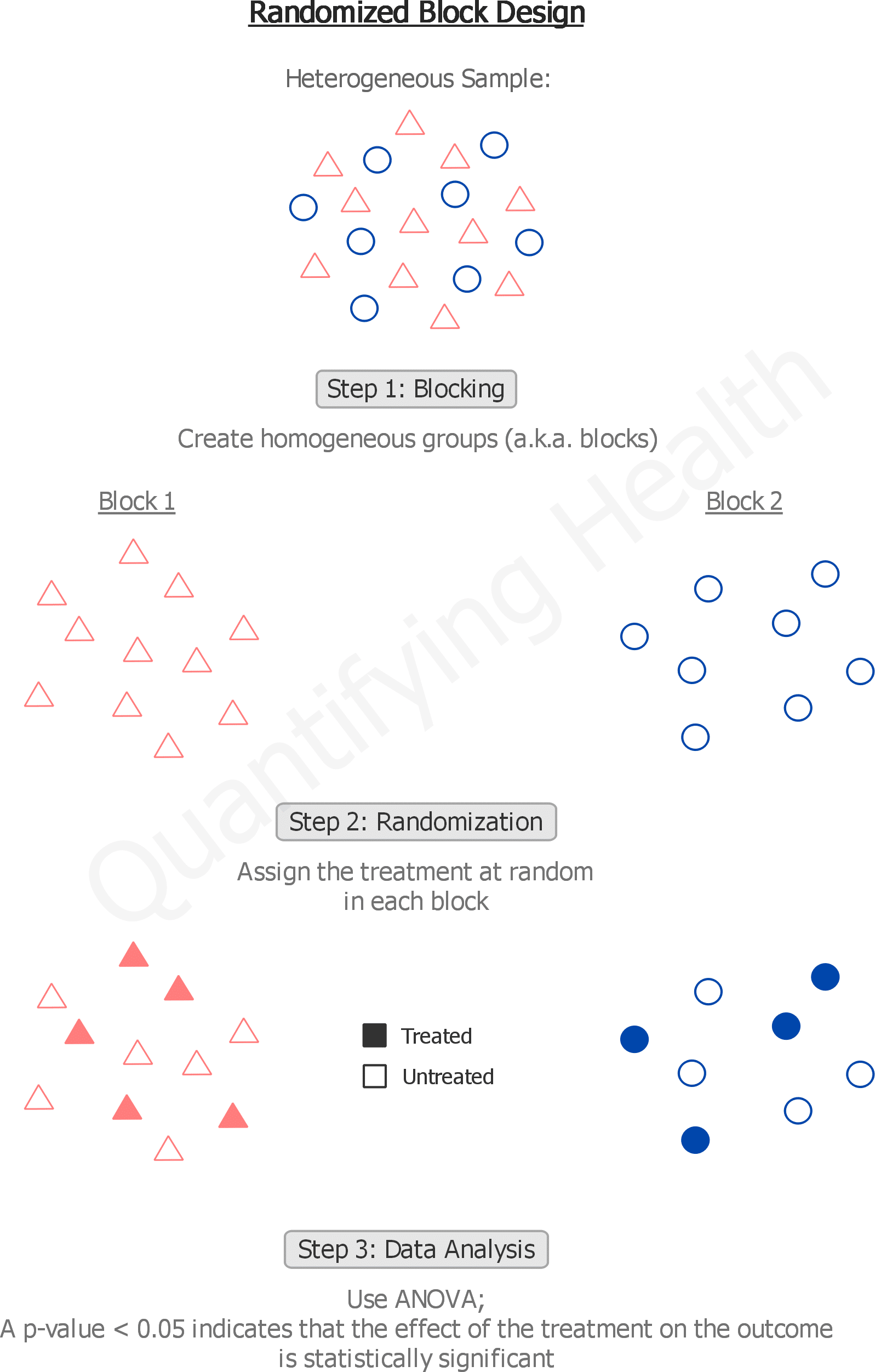
Many industrial and human subjects experiments involve blocking, or when they do not, probably should in order to reduce the unexplained variation. Here are the main steps you need to take in order to implement blocking in your experimental design. Blocking is one of those concepts that can be difficult to grasp even if you have already been exposed to it once or twice. Because the specific details of how blocking is implemented can vary a lot from one experiment to another.


No comments:
Post a Comment